LOAM源代码中坐标变换部分的详细讲解

作者：K.Fire

写在前面

本系列文章将对LOAM源代码进行讲解，在讲解过程中，涉及到论文中提到的部分，会结合论文以及我自己的理解进行解读，尤其是对于其中坐标变换的部分，将会进行详细的讲解。

本来是懒得写的，一个是怕自己以后忘了，另外是我在学习过程中，其实没有感觉哪一个博主能讲解的通篇都能让我很明白，特别是坐标变换部分的代码，所以想着自己学完之后，按照自己的理解，也写一个LOAM解读，希望能对后续学习LOAM的同学们有所帮助。

整体框架

LOAM多牛逼就不用多说了，直接开始

先贴一下我详细注释的LOAM代码，在这个版本的代码上加入了我自己的理解。

我觉得最重要也是最恶心的一部分是其中的坐标变换，在代码里面真的看着头大，所以先明确一下坐标系(都是右手坐标系)：

IMU(IMU坐标系imu)：x轴向前，y轴向左，z轴向上

LIDAR(激光雷达坐标系l)：x轴向前，y轴向左，z轴向上

CAMERA(相机坐标系，也可以理解为里程计坐标系c)：z轴向前，x轴向左，y轴向上

WORLD(世界坐标系w，也叫全局坐标系，与里程计第一帧init重合)：z轴向前，x轴向左，y轴向上

MAP(地图坐标系map，一定程度上可以理解为里程计第一帧init)：z轴向前，x轴向左，y轴向上

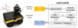
坐标变换约定： 为了清晰，变换矩阵的形式与《SLAM十四讲中一样》，即：表示B坐标系相对于A坐标系的变换，B中一个向量通过可以变换到A中的向量。首先对照ros的节点图和论文中提到的算法框架来看一下：

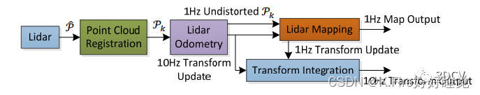
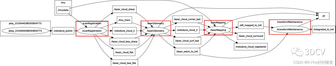
可以看到节点图和论文中的框架是一一对应的，这几个模块的功能如下：

scanRegistration：对原始点云进行预处理，计算曲率，提取特征点

laserOdometry：对当前sweep与上一次sweep进行特征匹配，计算一个快速(10Hz)但粗略的位姿估计

laserMapping：对当前sweep与一个局部子图进行特征匹配，计算一个慢速(1Hz)比较精确的位姿估计

transformMaintenance：对两个模块计算出的位姿进行融合，得到最终的精确地位姿估计

本文介绍laserOdometry模块，它相当于SLAM的前端，它其实是一个scan-to-scan的过程，可以得到高频率但精度略低的位姿变换，它的具体功能如下：

接收特征点话题、全部点云话题、IMU话题，并保存到对应的变量中

将当前sweep与上一次sweep进行特征匹配，得到edge point匹配对应的直线以及planar point匹配对应的平面

计算雅可比矩阵，使用高斯牛顿法(论文中说的是LM法)进行优化，得到估计出的相邻两帧的位姿变换

累积位姿变换，并用IMU修正，得到当前帧到初始帧的累积位姿变换

发布话题并更新tf变换

一、main()函数以及回调函数

main()函数是很简单的，就是定义了一系列的发布者和订阅者，订阅了来自scanRegistration节点发布的话题；然后定义了一个tf发布器，发布当前帧(/laser_odom)到初始帧(/camera_init)的坐标变换；然后定义了一些列下面会用到的变量。

其中有6个订阅者，分别看一下它们的回调函数。

intmain(intargc,char**argv)
{
ros::init(argc,argv,"laserOdometry");
ros::NodeHandlenh;

ros::SubscribersubCornerPointsSharp=nh.subscribe
("/laser_cloud_sharp",2,laserCloudSharpHandler);

ros::SubscribersubCornerPointsLessSharp=nh.subscribe
("/laser_cloud_less_sharp",2,laserCloudLessSharpHandler);

ros::SubscribersubSurfPointsFlat=nh.subscribe
("/laser_cloud_flat",2,laserCloudFlatHandler);

ros::SubscribersubSurfPointsLessFlat=nh.subscribe
("/laser_cloud_less_flat",2,laserCloudLessFlatHandler);

ros::SubscribersubLaserCloudFullRes=nh.subscribe
("/velodyne_cloud_2",2,laserCloudFullResHandler);

ros::SubscribersubImuTrans=nh.subscribe
("/imu_trans",5,imuTransHandler);

ros::PublisherpubLaserCloudCornerLast=nh.advertise
("/laser_cloud_corner_last",2);

ros::PublisherpubLaserCloudSurfLast=nh.advertise
("/laser_cloud_surf_last",2);

ros::PublisherpubLaserCloudFullRes=nh.advertise
("/velodyne_cloud_3",2);

ros::PublisherpubLaserOdometry=nh.advertise("/laser_odom_to_init",5);
nav_msgs::OdometrylaserOdometry;
laserOdometry.header.frame_id="/camera_init";
laserOdometry.child_frame_id="/laser_odom";

tf::TransformBroadcastertfBroadcaster;
tf::StampedTransformlaserOdometryTrans;
laserOdometryTrans.frame_id_="/camera_init";
laserOdometryTrans.child_frame_id_="/laser_odom";

std::vectorpointSearchInd;//搜索到的点序
std::vectorpointSearchSqDis;//搜索到的点平方距离

PointTypepointOri,pointSel;/*选中的特征点*/
PointTypetripod1,tripod2,tripod3;/*特征点的对应点*/
PointTypepointProj;/*unused*/
PointTypecoeff;/*直线或平面的系数*/

//退化标志
boolisDegenerate=false;
//P矩阵，预测矩阵，用来处理退化情况
cv::MatmatP(6,6,CV_32F,cv::all(0));

intframeCount=skipFrameNum;//skipFrameNum=1
ros::Raterate(100);
boolstatus=ros::ok();

接收特征点的回调函数

下面这五个回调函数的作用和代码结构都类似，都是接收scanRegistration发布的话题，分别接收了edge point、less edge point、planar point、less planar point、full cloud point(按scanID排列的全部点云)。

对于接收到点云之后都是如下操作：

记录时间戳

保存到相应变量中

滤除无效点

将接收标志设置为true

voidlaserCloudSharpHandler(constsensor_msgs::PointCloud2ConstPtr&cornerPointsSharp2)
{
timeCornerPointsSharp=cornerPointsSharp2->header.stamp.toSec();

cornerPointsSharp->clear();
pcl::fromROSMsg(*cornerPointsSharp2,*cornerPointsSharp);
std::vectorindices;
pcl::removeNaNFromPointCloud(*cornerPointsSharp,*cornerPointsSharp,indices);
newCornerPointsSharp=true;
}

voidlaserCloudLessSharpHandler(constsensor_msgs::PointCloud2ConstPtr&cornerPointsLessSharp2)
{
timeCornerPointsLessSharp=cornerPointsLessSharp2->header.stamp.toSec();

cornerPointsLessSharp->clear();
pcl::fromROSMsg(*cornerPointsLessSharp2,*cornerPointsLessSharp);
std::vectorindices;
pcl::removeNaNFromPointCloud(*cornerPointsLessSharp,*cornerPointsLessSharp,indices);
newCornerPointsLessSharp=true;
}

voidlaserCloudFlatHandler(constsensor_msgs::PointCloud2ConstPtr&surfPointsFlat2)
{
timeSurfPointsFlat=surfPointsFlat2->header.stamp.toSec();

surfPointsFlat->clear();
pcl::fromROSMsg(*surfPointsFlat2,*surfPointsFlat);
std::vectorindices;
pcl::removeNaNFromPointCloud(*surfPointsFlat,*surfPointsFlat,indices);
newSurfPointsFlat=true;
}

voidlaserCloudLessFlatHandler(constsensor_msgs::PointCloud2ConstPtr&surfPointsLessFlat2)
{
timeSurfPointsLessFlat=surfPointsLessFlat2->header.stamp.toSec();

surfPointsLessFlat->clear();
pcl::fromROSMsg(*surfPointsLessFlat2,*surfPointsLessFlat);
std::vectorindices;
pcl::removeNaNFromPointCloud(*surfPointsLessFlat,*surfPointsLessFlat,indices);
newSurfPointsLessFlat=true;
}

//接收全部点
voidlaserCloudFullResHandler(constsensor_msgs::PointCloud2ConstPtr&laserCloudFullRes2)
{
timeLaserCloudFullRes=laserCloudFullRes2->header.stamp.toSec();

laserCloudFullRes->clear();
pcl::fromROSMsg(*laserCloudFullRes2,*laserCloudFullRes);
std::vectorindices;
pcl::removeNaNFromPointCloud(*laserCloudFullRes,*laserCloudFullRes,indices);
newLaserCloudFullRes=true;
}

接收/imu_trans消息这个回调函数主要是接受了scanRegistration中发布的自定义imu话题，包括当前sweep点云数据的IMU起始角、终止角、由于加减速产生的位移和速度畸变，保存到相应变量中。

//接收imu消息
voidimuTransHandler(constsensor_msgs::PointCloud2ConstPtr&imuTrans2)
{
timeImuTrans=imuTrans2->header.stamp.toSec();

imuTrans->clear();
pcl::fromROSMsg(*imuTrans2,*imuTrans);

//根据发来的消息提取imu信息
imuPitchStart=imuTrans->points[0].x;
imuYawStart=imuTrans->points[0].y;
imuRollStart=imuTrans->points[0].z;

imuPitchLast=imuTrans->points[1].x;
imuYawLast=imuTrans->points[1].y;
imuRollLast=imuTrans->points[1].z;

imuShiftFromStartX=imuTrans->points[2].x;
imuShiftFromStartY=imuTrans->points[2].y;
imuShiftFromStartZ=imuTrans->points[2].z;

imuVeloFromStartX=imuTrans->points[3].x;
imuVeloFromStartY=imuTrans->points[3].y;
imuVeloFromStartZ=imuTrans->points[3].z;

newImuTrans=true;
}

二、特征匹配

2.1 初始化

接收到第一帧点云数据时，先进行一次初始化，因为第一帧点云没法匹配..

这里就是直接把这一帧点云发送给laserMapping节点。

//初始化：将第一个点云数据集发送给laserMapping,从下一个点云数据开始处理
if(!systemInited){
//将cornerPointsLessSharp与laserCloudCornerLast交换,目的保存cornerPointsLessSharp的值到laserCloudCornerLast中下轮使用
pcl::PointCloud::PtrlaserCloudTemp=cornerPointsLessSharp;
cornerPointsLessSharp=laserCloudCornerLast;
laserCloudCornerLast=laserCloudTemp;

//将surfPointLessFlat与laserCloudSurfLast交换，目的保存surfPointsLessFlat的值到laserCloudSurfLast中下轮使用
laserCloudTemp=surfPointsLessFlat;
surfPointsLessFlat=laserCloudSurfLast;
laserCloudSurfLast=laserCloudTemp;

//使用上一帧的特征点构建kd-tree
kdtreeCornerLast->setInputCloud(laserCloudCornerLast);//所有的边沿点集合
kdtreeSurfLast->setInputCloud(laserCloudSurfLast);//所有的平面点集合

//将cornerPointsLessSharp和surfPointLessFlat点也即边沿点和平面点分别发送给laserMapping
sensor_msgs::PointCloud2laserCloudCornerLast2;
pcl::toROSMsg(*laserCloudCornerLast,laserCloudCornerLast2);
laserCloudCornerLast2.header.stamp=ros::Time().fromSec(timeSurfPointsLessFlat);
laserCloudCornerLast2.header.frame_id="/camera";
pubLaserCloudCornerLast.publish(laserCloudCornerLast2);

sensor_msgs::PointCloud2laserCloudSurfLast2;
pcl::toROSMsg(*laserCloudSurfLast,laserCloudSurfLast2);
laserCloudSurfLast2.header.stamp=ros::Time().fromSec(timeSurfPointsLessFlat);
laserCloudSurfLast2.header.frame_id="/camera";
pubLaserCloudSurfLast.publish(laserCloudSurfLast2);

//记住原点的翻滚角和俯仰角
transformSum[0]+=imuPitchStart;//IMU的y方向
transformSum[2]+=imuRollStart;//IMU的x方向

systemInited=true;
continue;
}

2.2 TransformToStart()函数

在scanRegistration模块中，有一个TransformToStartIMU()函数，上篇文章提到它的作用是：没有对点云坐标系进行变换，第i个点云依然处在里程计坐标系下的curr时刻坐标系中，只是对点云的位置进行调整。在这里推荐工坊新课：（第二期）彻底搞懂基于LOAM框架的3D激光SLAM：源码剖析到算法优化

而这个函数呢，就是要对点云的坐标系进行变换，变换到里程计坐标系下的初始时刻start坐标系中，用于与上一帧的点云数据进行匹配。

在这个函数中，首先根据每个点强度值intensity，提取出scanRegistration中计算的插值系数，下面开始了！

首先要明确：transform中保存的变量是上一帧相对于当前帧的变换，也就是

而这里也体现了匀速运动假设，因为我们在这里使用transform变量时，还没有对其进行更新(迭代更新过程在特征匹配和非线性最小二乘优化中才进行)，所以这里使用的transform变量与上上帧相对于上一帧的变换相同，这也就是作者假设了每个扫描周期车辆都进行了完全相同的运动，用数学公式表示如下：

那么问题如下：

现在我们已知的量是：当前时刻坐标系下保持imustart角的的点云，上一帧相对于当前帧的变换，也就是，使用s进行插值后有：。

需要求解的是当前sweep初始时刻坐标系的点云。

推导过程：

根据坐标变换公式有：

而为YXZ变换顺序(解释：当前帧相对于上一帧的变换顺序为ZXY，呢么反过来，这里是上一帧相当于当前帧的变换，就变成了YXZ)，所以，代入得：

这就推出了和代码一致的变换顺序：先减去，然后绕z周旋转-rz，绕x轴旋转-rx，绕y轴旋转-ry。

//将该次sweep中每个点通过插值，变换到初始时刻start
voidTransformToStart(PointTypeconst*constpi,PointType*constpo)
{
//插值系数计算，云中每个点的相对时间/点云周期10
floats=10*(pi->intensity-int(pi->intensity));

//线性插值：根据每个点在点云中的相对位置关系，乘以相应的旋转平移系数
//这里的transform数值上和上次一样，这里体现了匀速运动模型，就是每次时间间隔下，相对于上一次sweep的变换都是一样的
//而在使用该函数之前进行了一次操作：transform[3]-=imuVeloFromStartX*scanPeriod;
//这个操作是在匀速模型的基础上，去除了由于加减速造成的畸变

//R_curr_start=R_YXZ
floatrx=s*transform[0];
floatry=s*transform[1];
floatrz=s*transform[2];
floattx=s*transform[3];
floatty=s*transform[4];
floattz=s*transform[5];

/*pi是在curr坐标系下p_curr，需要变换到当前sweep的初始时刻start坐标系下
*现在有关系：p_curr=R_curr_start*p_start+t_curr_start
*变换一下有：变换一下有：p_start=R_curr_start^{-1}*(p_curr-t_curr_start)=R_YXZ^{-1}*(p_curr-t_curr_start)
*代入定义量：p_start=R_transform^{-1}*(p_curr-t_transform)
*展开已知角：p_start=R_-ry*R_-rx*R_-rz*(p_curr-t_transform)
*/

//平移后绕z轴旋转（-rz）
floatx1=cos(rz)*(pi->x-tx)+sin(rz)*(pi->y-ty);
floaty1=-sin(rz)*(pi->x-tx)+cos(rz)*(pi->y-ty);
floatz1=(pi->z-tz);

//绕x轴旋转（-rx）
floatx2=x1;
floaty2=cos(rx)*y1+sin(rx)*z1;
floatz2=-sin(rx)*y1+cos(rx)*z1;

//绕y轴旋转（-ry）
po->x=cos(ry)*x2-sin(ry)*z2;
po->y=y2;
po->z=sin(ry)*x2+cos(ry)*z2;
po->intensity=pi->intensity;
}

2.2 edge point匹配

寻找匹配直线：

将该次sweep中每个点通过插值，变换到初始时刻start后，迭代五次时，重新查找最近点，相当于每个匹配迭代优化4次，A-LOAM代码中的Ceres代码的最大迭代次数为4。

然后先试用PCL中的KD-tree查找当前点在上一帧中的最近邻点，对应论文中提到的j点，最近邻在上一帧中的索引保存在pointSearchInd中，距离保存在pointSearchSqDis中。

kdtreeCornerLast->nearestKSearch(pointSel, 1, pointSearchInd, pointSearchSqDis);

closestPointInd对应论文中的j点，minPointInd2对应论文中的l点

int closestPointInd = -1, minPointInd2 = -1;

如果查找到了最近邻的j点，就按照论文中所说，需要查找上一帧中，与j线号scanID相邻且j的最近邻点l，j和l构成与待匹配点i的匹配直线edge。

下面这两个for循环做了这么一件事情：向索引增大的方向查找(scanID>=j点的scanID)，如果查找到了相邻帧有距离更小的点，就更新最小距离和索引；然后向索引减小的方向查找(scanID<=j点的scanID)，如果查找到了相邻帧有距离更小的点，就更新最小距离和索引。然后将每个待匹配点对应的j和l点的索引保存在pointSearchCornerInd1[]和pointSearchCornerInd2[]中。

计算直线参数：

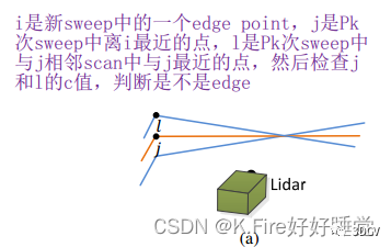
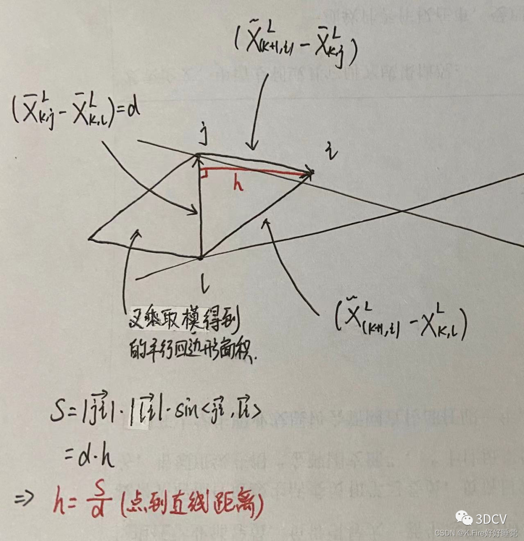
当找到了j点和l点，就可以进行特征匹配，计算匹配直线的系数，对应论文中的公式为：

这个公式的分子是i和j构成的向量与i和l构成的向量的叉乘，得到了一个与ijl三点构成平面垂直的向量，而叉乘取模其实就是一个平行四边形面积；分母是j和l构成的向量，取模后为平行四边形面积的底，二者相除就得到了i到直线jl的距离，下面是图示：

代码中变量代表的含义：

x0：i点

x1：j点

x2：l点

a012：论文中残差的分子(两个向量的叉乘)

la、lb、lc：i点到jl线垂线方向的向量(jl方向的单位向量与ijl平面的单位法向量的叉乘得到)在xyz三个轴上的分量

ld2：点到直线的距离，即

下面这个s可以看做一个权重，距离越大权重越小，距离越小权重越大，得到的权重范围<=1,其实就是在求解非线性最小二乘问题时的核函数，s的本质定义如下：

最后将权重大(>0.1)的，即距离比较小，且距离不为零的点放入laserCloudOri，对应的直线系数放入coeffSel。

//论文中提到的Levenberg-Marquardt算法(L-Mmethod)，其实是高斯牛顿算法
for(intiterCount=0;iterCount< 25; iterCount++) {
          laserCloudOri->clear();
coeffSel->clear();

//处理当前点云中的曲率最大的特征点,从上个点云中曲率比较大的特征点中找两个最近距离点，一个点使用kd-tree查找，另一个根据找到的点在其相邻线找另外一个最近距离的点
for(inti=0;i< cornerPointsSharpNum; i++) {
            //将该次sweep中每个点通过插值，变换到初始时刻start
            TransformToStart(&cornerPointsSharp->points[i],&pointSel);

//每迭代五次，重新查找最近点，相当于每个匹配迭代优化4次，ALOAM代码中的Ceres代码的最大迭代次数为4
if(iterCount%5==0){
std::vectorindices;
pcl::removeNaNFromPointCloud(*laserCloudCornerLast,*laserCloudCornerLast,indices);
//kd-tree查找一个最近距离点，边沿点未经过体素栅格滤波，一般边沿点本来就比较少，不做滤波
kdtreeCornerLast->nearestKSearch(pointSel,1,pointSearchInd,pointSearchSqDis);
intclosestPointInd=-1,minPointInd2=-1;
//closestPointInd对应论文中的j点，minPointInd2对应论文中的l点

//循环是寻找相邻线最近点l
//再次提醒：velodyne是2度一线，scanID相邻并不代表线号相邻，相邻线度数相差2度，也即线号scanID相差2
if(pointSearchSqDis[0]< 25) {//找到的最近点距离的确很近的话
                closestPointInd = pointSearchInd[0];
                //提取最近点线号
                int closestPointScan = int(laserCloudCornerLast->points[closestPointInd].intensity);

floatpointSqDis,minPointSqDis2=25;//初始门槛值25米，可大致过滤掉scanID相邻，但实际线不相邻的值
//寻找距离目标点最近距离的平方和最小的点
for(intj=closestPointInd+1;j< cornerPointsSharpNum; j++) {//向scanID增大的方向查找
                  if (int(laserCloudCornerLast->points[j].intensity)>closestPointScan+2.5){//非相邻线
break;
}
...

2.3 planar point匹配

寻找匹配平面：

将该次sweep中每个点通过插值，变换到初始时刻start后，迭代五次时，重新查找最近点，相当于每个匹配迭代优化4次，A-LOAM代码中的Ceres代码的最大迭代次数为4。

然后先试用PCL中的KD-tree查找当前点在上一帧中的最近邻点，对应论文中提到的j点，最近邻在上一帧中的索引保存在pointSearchInd中，距离保存在pointSearchSqDis中。

kdtreeCornerLast->nearestKSearch(pointSel, 1, pointSearchInd, pointSearchSqDis);

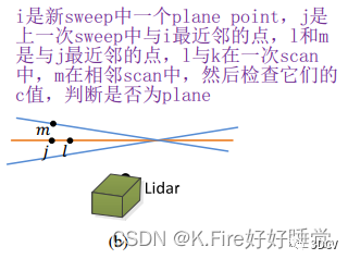
closestPointInd对应论文中的j点、minPointInd2对应论文中的l点、minPointInd3对应论文中的m点。

int closestPointInd = -1, minPointInd2 = -1, minPointInd3 = -1;

如果查找到了最近邻的j点，就按照论文中所说，需要查找上一帧中，与j线号scanID相同且j的最近邻点l，然后查找一个与j线号scanID相邻且最近邻的点m。

下面这两个for循环做了这么一件事情：向索引增大的方向查找(scanID>=j点的scanID)，如果查找到了相邻线号的点j和相同线号的点m，有距离更小的点，就更新最小距离和索引；然后向索引减小的方向查找(scanID<=j点的scanID)，如果查找到了相邻线号的点j和相同线号的点m，就更新最小距离和索引。然后将每个待匹配点对应的j、l点、m点的索引保存在pointSearchSurfInd1[]、pointSearchSurfInd2[]和pointSearchSurfInd3[]中。

计算平面参数：

当找到了j点、l点和m点，就可以进行特征匹配，计算匹配直线的系数，对应论文中的公式为：

这个公式的分母是一个lj向量和mj向量叉乘的形式，表示的是jlm平面的法向量的模；而分子是ij向量与jlm平面的法向量的向量积，向量积有一个意义是一个向量在另一个向量方向上的投影，这里就表示ij向量在jlm平面的法向量方向上的投影，也就是i到平面的距离，下面是图示：

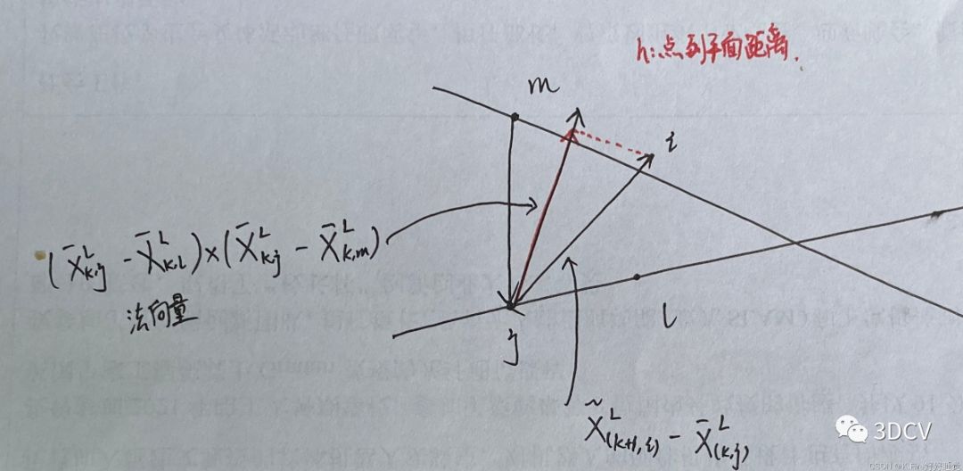
代码中变量代表的含义：

tripod1：j点

tripod2：l点

tripod3：m点

pa、pb、pc：jlm平面的法向量在xyz三个轴上的分量，也可以理解为平面方程Ax+By+Cz+D=0的ABC系数

pd：为平面方程的D系数

ps：法向量的模

pd2：点到平面的距离(将平面方程的系数归一化后，代入点的坐标，其实就是点到平面距离公式，即可得到点到平面的距离)

下面这个s可以看做一个权重，对应于论文中的这一部分

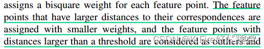
距离越大权重越小，距离越小权重越大，得到的权重范围<=1,其实就是在求解非线性最小二乘问题时的核函数，s的本质定义如下：

最后将权重大(>0.1)的，即距离比较小，且距离不为零的点放入laserCloudOri，对应的平面系数放入coeffSel。

//对本次接收到的曲率最小的点,从上次接收到的点云曲率比较小的点中找三点组成平面，一个使用kd-tree查找，另外一个在同一线上查找满足要求的，第三个在不同线上查找满足要求的
for(inti=0;i< surfPointsFlatNum; i++) {
            //将该次sweep中每个点通过插值，变换到初始时刻start
            TransformToStart(&surfPointsFlat->points[i],&pointSel);

if(iterCount%5==0){
//kd-tree最近点查找，在经过体素栅格滤波之后的平面点中查找，一般平面点太多，滤波后最近点查找数据量小
kdtreeSurfLast->nearestKSearch(pointSel,1,pointSearchInd,pointSearchSqDis);

//closestPointInd对应论文中的j、minPointInd2对应论文中的l、minPointInd3对应论文中的m
intclosestPointInd=-1,minPointInd2=-1,minPointInd3=-1;
if(pointSearchSqDis[0]< 25) {
                closestPointInd = pointSearchInd[0];
                int closestPointScan = int(laserCloudSurfLast->points[closestPointInd].intensity);

floatpointSqDis,minPointSqDis2=25,minPointSqDis3=25;
for(intj=closestPointInd+1;j< surfPointsFlatNum; j++) { //向上查找
                  if (int(laserCloudSurfLast->points[j].intensity)>closestPointScan+2.5){
break;
}

...

三、高斯牛顿优化

3.1 计算雅可比矩阵并求解增量

在代码中，作者是纯手推的高斯牛顿算法，这种方式相比于使用Ceres等工具，会提高运算速度，但是计算雅克比矩阵比较麻烦，需要清晰的思路和扎实的数学功底，下面我们一起来推导一下。

以edge point匹配为例，planar point是一样的。

设误差函数(点到直线的距离)为：

其中，X为待优化变量，也就是transform[6]中存储的变量，表示3轴旋转rx、ry、rz和3轴平移量tx、ty、tz；D()表示两点之间的距离，其计算公式为：

表示start时刻坐标系下待匹配点i；表示start时刻坐标系下点i到直线jl的垂点；另外根据之前TransformToStart()函数推导过的坐标变换有：

根据链式法则，f(x)对X求导有：

对其中每一项进行计算：

D对求导的结果其实就是 进行归一化后的点到直线向量，它在xyz三个轴的分量就是前面求解出来的la、lb、lc变量。

用上面的结果，分别对rx,ry,rz,tx,ty,tz求导，将得到的结果(3x6矩阵)再与D对求导的结果(1x3矩阵)相乘，就可以得到代码中显示的结果(1x6矩阵)，分别赋值到matA的6个位置，matB是残差项。

最后使用opencv的QR分解求解增量X即可。

//满足要求的特征点至少10个，特征匹配数量太少弃用此帧数据，不再进行优化步骤
if(pointSelNum< 10) {
            continue;
          }

          // Hx=g
          cv::Mat matA(pointSelNum, 6, CV_32F, cv::all(0));     // J
          cv::Mat matAt(6, pointSelNum, CV_32F, cv::all(0));    // J^T
          cv::Mat matAtA(6, 6, CV_32F, cv::all(0));             // H = J^T * J
          cv::Mat matB(pointSelNum, 1, CV_32F, cv::all(0));     // e
          cv::Mat matAtB(6, 1, CV_32F, cv::all(0));             // g = -J * e
          cv::Mat matX(6, 1, CV_32F, cv::all(0));               // x

          //计算matA,matB矩阵
          for (int i = 0; i < pointSelNum; i++) {
            pointOri = laserCloudOri->points[i];
coeff=coeffSel->points[i];

floats=1;

floatsrx=sin(s*transform[0]);
floatcrx=cos(s*transform[0]);
floatsry=sin(s*transform[1]);
floatcry=cos(s*transform[1]);
floatsrz=sin(s*transform[2]);
floatcrz=cos(s*transform[2]);
floattx=s*transform[3];
floatty=s*transform[4];
floattz=s*transform[5];

floatarx=(-s*crx*sry*srz*pointOri.x+s*crx*crz*sry*pointOri.y+s*srx*sry*pointOri.z
+s*tx*crx*sry*srz-s*ty*crx*crz*sry-s*tz*srx*sry)*coeff.x
+(s*srx*srz*pointOri.x-s*crz*srx*pointOri.y+s*crx*pointOri.z
+s*ty*crz*srx-s*tz*crx-s*tx*srx*srz)*coeff.y
+(s*crx*cry*srz*pointOri.x-s*crx*cry*crz*pointOri.y-s*cry*srx*pointOri.z
+s*tz*cry*srx+s*ty*crx*cry*crz-s*tx*crx*cry*srz)*coeff.z;

floatary=((-s*crz*sry-s*cry*srx*srz)*pointOri.x
+(s*cry*crz*srx-s*sry*srz)*pointOri.y-s*crx*cry*pointOri.z
+tx*(s*crz*sry+s*cry*srx*srz)+ty*(s*sry*srz-s*cry*crz*srx)
+s*tz*crx*cry)*coeff.x
+((s*cry*crz-s*srx*sry*srz)*pointOri.x
+(s*cry*srz+s*crz*srx*sry)*pointOri.y-s*crx*sry*pointOri.z
+s*tz*crx*sry-ty*(s*cry*srz+s*crz*srx*sry)
-tx*(s*cry*crz-s*srx*sry*srz))*coeff.z;

floatarz=((-s*cry*srz-s*crz*srx*sry)*pointOri.x+(s*cry*crz-s*srx*sry*srz)*pointOri.y
+tx*(s*cry*srz+s*crz*srx*sry)-ty*(s*cry*crz-s*srx*sry*srz))*coeff.x
+(-s*crx*crz*pointOri.x-s*crx*srz*pointOri.y
+s*ty*crx*srz+s*tx*crx*crz)*coeff.y
+((s*cry*crz*srx-s*sry*srz)*pointOri.x+(s*crz*sry+s*cry*srx*srz)*pointOri.y
+tx*(s*sry*srz-s*cry*crz*srx)-ty*(s*crz*sry+s*cry*srx*srz))*coeff.z;

floatatx=-s*(cry*crz-srx*sry*srz)*coeff.x+s*crx*srz*coeff.y
-s*(crz*sry+cry*srx*srz)*coeff.z;

floataty=-s*(cry*srz+crz*srx*sry)*coeff.x-s*crx*crz*coeff.y
-s*(sry*srz-cry*crz*srx)*coeff.z;

floatatz=s*crx*sry*coeff.x-s*srx*coeff.y-s*crx*cry*coeff.z;

floatd2=coeff.intensity;

matA.at(i,0)=arx;
matA.at(i,1)=ary;
matA.at(i,2)=arz;
matA.at(i,3)=atx;
matA.at(i,4)=aty;
matA.at(i,5)=atz;
matB.at(i,0)=-0.05*d2;
}
cv::transpose(matA,matAt);
matAtA=matAt*matA;
matAtB=matAt*matB;
//求解matAtA*matX=matAtB
cv::solve(matAtA,matAtB,matX,cv::DECOMP_QR);

3.2 退化处理

代码中使用的退化处理在Ji Zhang的这篇论文(《On Degeneracy of Optimization-based State Estimation Problems》)中有详细论述。

简单来说，作者认为退化只可能发生在第一次迭代时，先对矩阵求特征值，然后将得到的特征值与阈值(代码中为10)进行比较，如果小于阈值则认为该特征值对应的特征向量方向发生了退化，将对应的特征向量置为0，然后按照论文中所述，计算一个P矩阵：

是原来的特征向量矩阵，是将退化方向置为0后的特征向量矩阵，然后用P矩阵与原来得到的解相乘，得到最终解：

if(iterCount==0){
//特征值1*6矩阵
cv::MatmatE(1,6,CV_32F,cv::all(0));
//特征向量6*6矩阵
cv::MatmatV(6,6,CV_32F,cv::all(0));
cv::MatmatV2(6,6,CV_32F,cv::all(0));

//求解特征值/特征向量
cv::eigen(matAtA,matE,matV);
matV.copyTo(matV2);

isDegenerate=false;
//特征值取值门槛
floateignThre[6]={10,10,10,10,10,10};
for(inti=5;i>=0;i--){//从小到大查找
if(matE.at(0,i)< eignThre[i]) {//特征值太小，则认为处在退化环境中，发生了退化
                for (int j = 0; j < 6; j++) {//对应的特征向量置为0
                  matV2.at(i,j)=0;
}
isDegenerate=true;
}else{
break;
}
}

//计算P矩阵
matP=matV.inv()*matV2;//论文中对应的Vf^-1*V_u`
}

if(isDegenerate){//如果发生退化，只使用预测矩阵P计算
cv::MatmatX2(6,1,CV_32F,cv::all(0));
matX.copyTo(matX2);
matX=matP*matX2;
}

3.3 迭代更新

最后进行迭代更新，如果更新量很小则终止迭代。

//累加每次迭代的旋转平移量
transform[0]+=matX.at(0,0);
transform[1]+=matX.at(1,0);
transform[2]+=matX.at(2,0);
transform[3]+=matX.at(3,0);
transform[4]+=matX.at(4,0);
transform[5]+=matX.at(5,0);

for(inti=0;i<6; i++){
            if(isnan(transform[i]))//判断是否非数字
              transform[i]=0;
          }
          //计算旋转平移量，如果很小就停止迭代
          float deltaR = sqrt(
                              pow(rad2deg(matX.at(0,0)),2)+
pow(rad2deg(matX.at(1,0)),2)+
pow(rad2deg(matX.at(2,0)),2));
floatdeltaT=sqrt(
pow(matX.at(3,0)*100,2)+
pow(matX.at(4,0)*100,2)+
pow(matX.at(5,0)*100,2));

if(deltaR< 0.1 && deltaT < 0.1) {//迭代终止条件
            break;
          }

再次总结一下整个流程：

一共迭代25次，每次分为edge point和planar point两个处理过程

每迭代5次时，重新寻找最近点

其他情况时，根据找到的最近点和待匹配点，计算匹配得到的直线和平面方程

根据计算匹配得到的直线和平面方程，计算雅可比矩阵，并求解迭代增量

如果是第一次迭代，判断是否发生退化

更新迭代增量，并判断终止条件

四、发布话题和坐标变换

4.1 发布话题

这一部分首先奖transformSum更新为修正后的值，然后将欧拉角转换成四元数，发布里程计话题、广播tf坐标变换，然后将点云的曲率比较大和比较小的点投影到扫描结束位置；如果当前帧特征点数量足够多，就将其插入到KD-tree中用于下一次特征匹配；然后发布话题，发布的话题有：

/laser_cloud_corner_last：曲率较大的点--less edge point

/laser_cloud_surf_last：曲率较小的点--less planar point

/velodyne_cloud_3：全部点云--full cloud point

/laser_odom_to_init：里程计坐标系下，当前时刻end相对于初始时刻的坐标变换

//得到世界坐标系下的转移矩阵
transformSum[0]=rx;
transformSum[1]=ry;
transformSum[2]=rz;
transformSum[3]=tx;
transformSum[4]=ty;
transformSum[5]=tz;

//欧拉角转换成四元数
geometry_msgs::QuaterniongeoQuat=tf::createQuaternionMsgFromRollPitchYaw(rz,-rx,-ry);

//publish四元数和平移量
laserOdometry.header.stamp=ros::Time().fromSec(timeSurfPointsLessFlat);
laserOdometry.pose.pose.orientation.x=-geoQuat.y;
laserOdometry.pose.pose.orientation.y=-geoQuat.z;
laserOdometry.pose.pose.orientation.z=geoQuat.x;
laserOdometry.pose.pose.orientation.w=geoQuat.w;
laserOdometry.pose.pose.position.x=tx;
laserOdometry.pose.pose.position.y=ty;
laserOdometry.pose.pose.position.z=tz;
pubLaserOdometry.publish(laserOdometry);

//广播新的平移旋转之后的坐标系(rviz)
laserOdometryTrans.stamp_=ros::Time().fromSec(timeSurfPointsLessFlat);
laserOdometryTrans.setRotation(tf::Quaternion(-geoQuat.y,-geoQuat.z,geoQuat.x,geoQuat.w));
laserOdometryTrans.setOrigin(tf::Vector3(tx,ty,tz));
tfBroadcaster.sendTransform(laserOdometryTrans);

//对点云的曲率比较大和比较小的点投影到扫描结束位置
intcornerPointsLessSharpNum=cornerPointsLessSharp->points.size();
for(inti=0;i< cornerPointsLessSharpNum; i++) {
        TransformToEnd(&cornerPointsLessSharp->points[i],&cornerPointsLessSharp->points[i]);
}

intsurfPointsLessFlatNum=surfPointsLessFlat->points.size();
for(inti=0;i< surfPointsLessFlatNum; i++) {
        TransformToEnd(&surfPointsLessFlat->points[i],&surfPointsLessFlat->points[i]);
}

frameCount++;
//点云全部点，每间隔一个点云数据相对点云最后一个点进行畸变校正
if(frameCount>=skipFrameNum+1){//skipFrameNum=1
intlaserCloudFullResNum=laserCloudFullRes->points.size();
for(inti=0;i< laserCloudFullResNum; i++) {
          TransformToEnd(&laserCloudFullRes->points[i],&laserCloudFullRes->points[i]);
}
}

//畸变校正之后的点作为last点保存等下个点云进来进行匹配
pcl::PointCloud::PtrlaserCloudTemp=cornerPointsLessSharp;
cornerPointsLessSharp=laserCloudCornerLast;
laserCloudCornerLast=laserCloudTemp;

laserCloudTemp=surfPointsLessFlat;
surfPointsLessFlat=laserCloudSurfLast;
laserCloudSurfLast=laserCloudTemp;

laserCloudCornerLastNum=laserCloudCornerLast->points.size();
laserCloudSurfLastNum=laserCloudSurfLast->points.size();
//点足够多就构建kd-tree，否则弃用此帧，沿用上一帧数据的kd-tree
if(laserCloudCornerLastNum>10&&laserCloudSurfLastNum>100){
kdtreeCornerLast->setInputCloud(laserCloudCornerLast);
kdtreeSurfLast->setInputCloud(laserCloudSurfLast);
}

//按照跳帧数publich边沿点，平面点以及全部点给laserMapping(每隔一帧发一次)
if(frameCount>=skipFrameNum+1){
frameCount=0;

sensor_msgs::PointCloud2laserCloudCornerLast2;
pcl::toROSMsg(*laserCloudCornerLast,laserCloudCornerLast2);
laserCloudCornerLast2.header.stamp=ros::Time().fromSec(timeSurfPointsLessFlat);
laserCloudCornerLast2.header.frame_id="/camera";
pubLaserCloudCornerLast.publish(laserCloudCornerLast2);

sensor_msgs::PointCloud2laserCloudSurfLast2;
pcl::toROSMsg(*laserCloudSurfLast,laserCloudSurfLast2);
laserCloudSurfLast2.header.stamp=ros::Time().fromSec(timeSurfPointsLessFlat);
laserCloudSurfLast2.header.frame_id="/camera";
pubLaserCloudSurfLast.publish(laserCloudSurfLast2);

sensor_msgs::PointCloud2laserCloudFullRes3;
pcl::toROSMsg(*laserCloudFullRes,laserCloudFullRes3);
laserCloudFullRes3.header.stamp=ros::Time().fromSec(timeSurfPointsLessFlat);
laserCloudFullRes3.header.frame_id="/camera";
pubLaserCloudFullRes.publish(laserCloudFullRes3);
}
}

status=ros::ok();
rate.sleep();
}

4.2 将点云变换到结束时刻end--TransformToEnd()函数

这里对应于论文中体到的，变换到下图所示的将变换到。

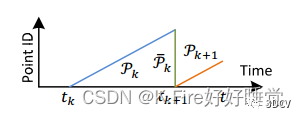
在匀速运动假设的前提下，从Start时刻到End时刻，点云都将保持imuRPYStart的位置姿态，然后对其中里程计坐标系下curr时刻的点进行以下操作：

1.首先进行了一个TransformToStart()函数的过程，将当前点变换到里程计坐标系下start时刻坐标系下，得到x3、y3、z3：

2.然后变换到里程计坐标系下end时刻坐标系下，再次提醒，得到x6、y6、z6：

但是事实上，由于加减速情况的存在，会产生运动畸变，这就导致匀速运动假设不再成立，也就是End时刻的imuRPY角与Start时刻的imuRPY角不相等，需要使用IMU去除畸变。

3.上面的过程，总体上看的结果就是将所有点保持imuRPYStrat的姿态，搬运到了雷达坐标系下的end时刻，由于运动畸变的存在，下面要使用IMU进行去畸变，首先将所有点转换到世界坐标系下，但仍然是里程计坐标系的end时刻，只是使用IMU进行了修正：

4.然后将所有点通过测量得到的imuRPYLast变换到全局(w)坐标系下的当前帧终止时刻，并且对应了imuRPYLast姿态角：

我理解的这个过程如下：

//将上一帧点云中的点相对结束位置去除因匀速运动产生的畸变，效果相当于得到在点云扫描结束位置静止扫描得到的点云
voidTransformToEnd(PointTypeconst*constpi,PointType*constpo)
{
//插值系数计算
floats=10*(pi->intensity-int(pi->intensity));

//R_curr_start
floatrx=s*transform[0];
floatry=s*transform[1];
floatrz=s*transform[2];
floattx=s*transform[3];
floatty=s*transform[4];
floattz=s*transform[5];

//将点curr系下的点，变换到初始时刻start
//平移后绕z轴旋转（-rz）
floatx1=cos(rz)*(pi->x-tx)+sin(rz)*(pi->y-ty);
floaty1=-sin(rz)*(pi->x-tx)+cos(rz)*(pi->y-ty);
floatz1=(pi->z-tz);

//绕x轴旋转（-rx）
floatx2=x1;
floaty2=cos(rx)*y1+sin(rx)*z1;
floatz2=-sin(rx)*y1+cos(rx)*z1;

//绕y轴旋转（-ry）
floatx3=cos(ry)*x2-sin(ry)*z2;
floaty3=y2;
floatz3=sin(ry)*x2+cos(ry)*z2;//求出了相对于起始点校正的坐标

//R_end_start=R_YXZ
rx=transform[0];
ry=transform[1];
rz=transform[2];
tx=transform[3];
ty=transform[4];
tz=transform[5];

//变换到end坐标系
//绕y轴旋转（ry）
floatx4=cos(ry)*x3+sin(ry)*z3;
floaty4=y3;
floatz4=-sin(ry)*x3+cos(ry)*z3;

//绕x轴旋转（rx）
floatx5=x4;
floaty5=cos(rx)*y4-sin(rx)*z4;
floatz5=sin(rx)*y4+cos(rx)*z4;

//绕z轴旋转（rz），再平移
floatx6=cos(rz)*x5-sin(rz)*y5+tx;
floaty6=sin(rz)*x5+cos(rz)*y5+ty;
floatz6=z5+tz;

//使用IMU去除由于加减速产生的运动畸变，然后变换到全局(w)坐标系下
//平移后绕z轴旋转（imuRollStart）
floatx7=cos(imuRollStart)*(x6-imuShiftFromStartX)
-sin(imuRollStart)*(y6-imuShiftFromStartY);
floaty7=sin(imuRollStart)*(x6-imuShiftFromStartX)
+cos(imuRollStart)*(y6-imuShiftFromStartY);
floatz7=z6-imuShiftFromStartZ;

//绕x轴旋转（imuPitchStart）
floatx8=x7;
floaty8=cos(imuPitchStart)*y7-sin(imuPitchStart)*z7;
floatz8=sin(imuPitchStart)*y7+cos(imuPitchStart)*z7;

//绕y轴旋转（imuYawStart）
floatx9=cos(imuYawStart)*x8+sin(imuYawStart)*z8;
floaty9=y8;
floatz9=-sin(imuYawStart)*x8+cos(imuYawStart)*z8;

//然后变换到全局(w)坐标系下的当前帧终止时刻
//绕y轴旋转（-imuYawLast）
floatx10=cos(imuYawLast)*x9-sin(imuYawLast)*z9;
floaty10=y9;
floatz10=sin(imuYawLast)*x9+cos(imuYawLast)*z9;

//绕x轴旋转（-imuPitchLast）
floatx11=x10;
floaty11=cos(imuPitchLast)*y10+sin(imuPitchLast)*z10;
floatz11=-sin(imuPitchLast)*y10+cos(imuPitchLast)*z10;

//绕z轴旋转（-imuRollLast）
po->x=cos(imuRollLast)*x11+sin(imuRollLast)*y11;
po->y=-sin(imuRollLast)*x11+cos(imuRollLast)*y11;
po->z=z11;
//只保留线号
po->intensity=int(pi->intensity);
}

总结

感觉如果去掉IMU的话，整个代码就很清晰，但是加上IMU部分就很容易让人懵逼。

编辑：黄飞